INDEX AND MATCH IN EXCEL

What is Index?

Index can be defined as a simple way of getting the value of a particular data from an array of table using row number and column number. It’s like a search tool that fetch out the specific value from a table array.

If you are able to follow the examples in this articles you will be able to use index and match in excel

Here is an example on how to use index in Excel:

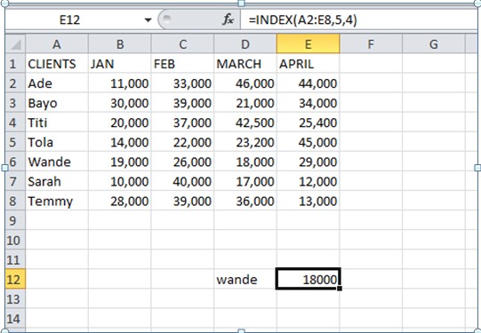
In the table below, we were told to give the value of client Wande’s sales in April using Index function.

Steps on how to use index function

1. Firstly write down the client’s name ( based on the question) as shown in cell D12.
2. Input an equal sign then type “index”, it will bring out the formular “ =Index( array, row_num, [ column_num]).
3. For the “array” you highlight the entire range of cells , for the “row_num” , locate client wande’s row ( i.e, client Wande is in row 5). For the column_num , locate the column where  April sales is ( i.e April sales is in column 5). Click on the “enter” key to get the value as shown in cell E12.

What is Match?

Match can be defined as a function in Excel that is used to know the row or column position of a particular data. Here is an example on how to use Match in Excel.

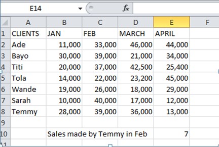
In the table below, we were told to locate the position of the sales made by client Temmy in February using Match function.

Steps on how to use Match function

1. Firstly write down what you are looking for in an empty cell as shown in cell D10
2. Input an equal sign then type “Match” , it will bring out the formular ( =match ( lookup_value, lookup_array, [ match type]).
3. For the “lookup_value”, you click on the lookup value you are looking for which is client Temmy, for the “lookup_array”, you highlight the drop down cell i.e the category in which you can find client Temmy. For the “match type” you will be given several options but since we want an exact match we will type 0 . Then click on the enter key.
4. AS shown in cellE10, the you will find the sales made by client Temmy in column7 which is 39,000

HOW TO USE THE COMBINATION OF BOTH INDEX AND MATCH

Using the example above, I will be using the combination of both the Index function and Match function to know the sales made by client Temmy in February.

Steps on how to use index and match

1. Start by typing the formula “=Index ( array i.e highlight everything for the array “ A2 to E8 “ then add the comma sign and move to the next argument.
2. This is where you will use the match function to specify the criteria. Type “match(” and enter the value you are looking as the “lookup_value , for the lookup_array highlight the category in which client Temmy is , select the match type which is 0 then close the match with a closing parenthesis ) , add a comma and input the column num which is 3 then add another closing  parenthesis and click on the enter key .
3. As shown in cell E10 below, the sales made by client  Temmy in Feb usingin the Index and Match function is 39,000

index and match in excel is one of the most important lookup and reference function that its combination helps us to use seach tool in locating a particular data from an array of table